FrozenLake RL

Classical RL Methods Checked against the Exact Optimum

Reinforcement learning · Oct 2026 · Completed

Fourteen classical RL methods on FrozenLake, Taxi and CliffWalking, each measured against the exact optimum computed from the model.

Dyna-Q optimal in 240 episodes
4 grid worlds

Built withPythonNumPyGymnasiumPyTorchMatplotlibpytest

View code on GitHub

Overview

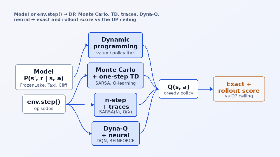
The toy-text environments in Gymnasium are small enough that the optimal policy can be computed exactly from the transition model, which makes them the right place to check whether a learning method actually works rather than guessing from noisy curves. I built one package where every classical method from Sutton and Barto runs through the same command: value and policy iteration, first-visit and every-visit Monte Carlo control, SARSA, expected SARSA, Q-learning, double Q-learning, n-step SARSA, SARSA(lambda) and Q(lambda) with eligibility traces, Dyna-Q, and DQN and REINFORCE on one-hot states.

Every method uses the same exploration schedule and the same two evaluations: an exact score of the greedy policy computed from the model within the time limit, and 1,000 real episodes. A finite-horizon dynamic program gives the ceiling for each environment, so each table reads as distance to the best possible policy. The same code draws value heatmaps, policy arrows, learning curves and the before/after animations.

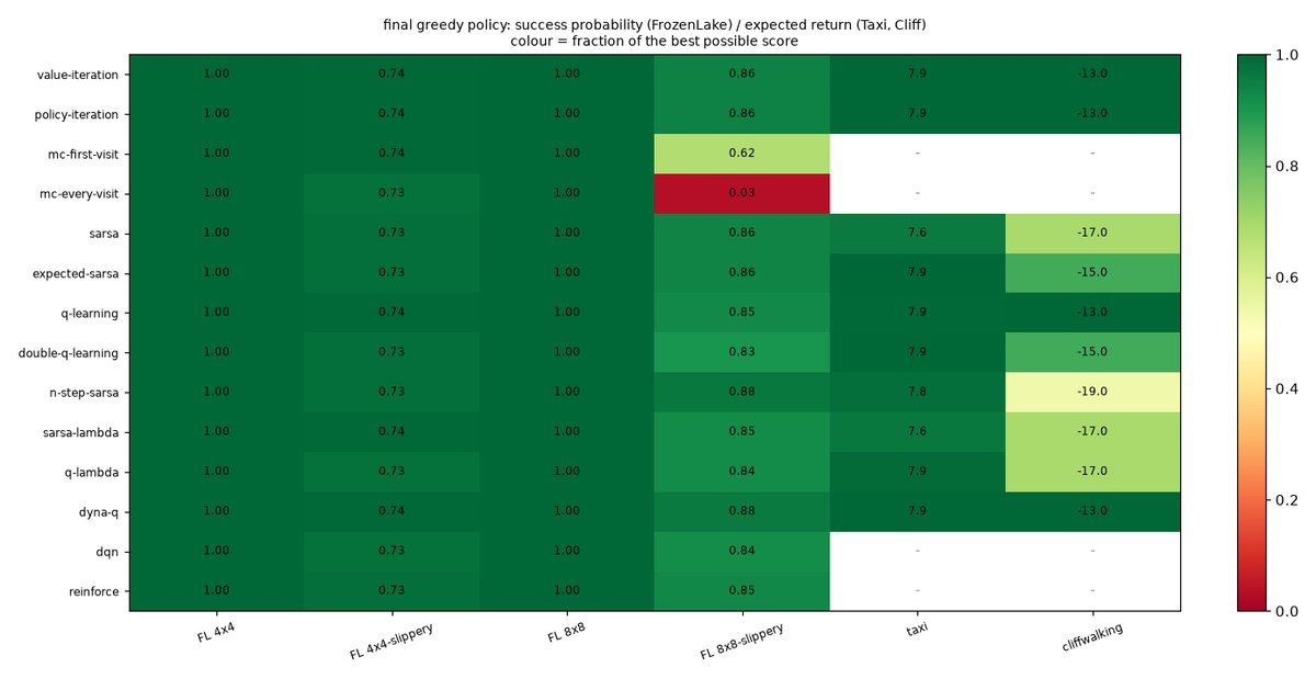
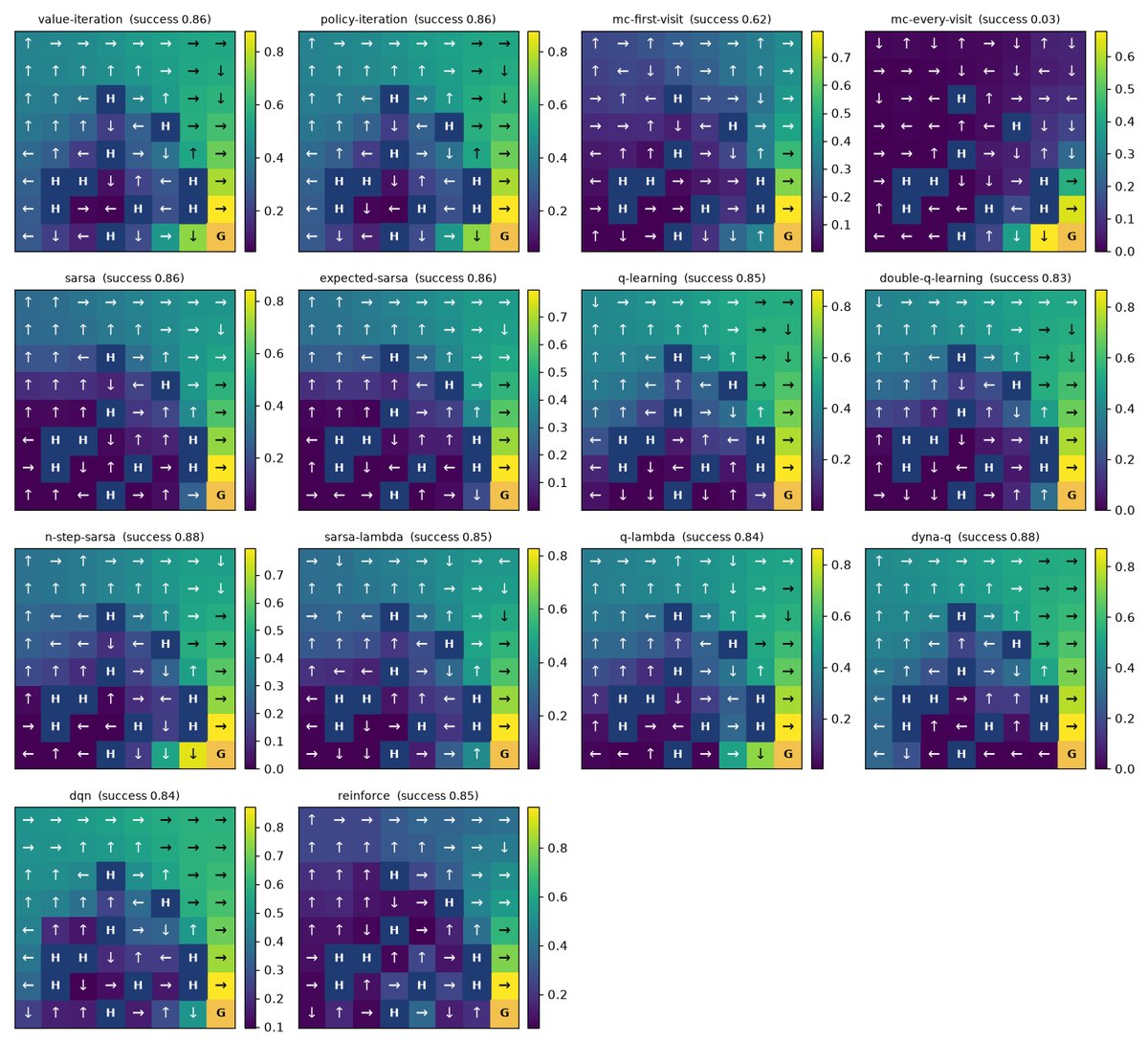
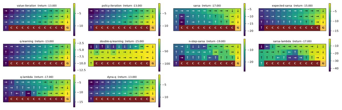
The runs confirm the textbook and put numbers on it. Every method reaches the optimum on the slippery 4x4 lake, but Dyna-Q needs 240 episodes where every-visit Monte Carlo needs 19,200. On the slippery 8x8 lake Monte Carlo fails outright (0.62 and 0.03 success) while TD methods reach 0.83-0.88. On CliffWalking, Q-learning finds the -13 edge path and SARSA keeps a safer -17 path, exactly as in example 6.6 of the book.

The question

When the problem is small enough that the optimal policy can be computed from the model, how close does each classical method get, and how many episodes does it need to get there?

Key features

Fourteen methods behind one --method flag, grouped as DP, Monte Carlo, TD, n-step and traces, planning and neural, on six environments: FrozenLake 4x4 and 8x8 with and without slipping, Taxi and CliffWalking.
Exact evaluation of any policy from the transition model P with the time limit, plus a 1,000-episode rollout evaluation that agrees with it within Monte Carlo error.
A finite-horizon DP ceiling per environment (0.744 and 0.913 on the slippery lakes, 7.93 on Taxi, -13 on CliffWalking) so every result is read as distance to optimal.
A Tracker that scores the greedy policy at 100 points per run and reports episodes to target, with learning curves and online training returns.
Value heatmaps, policy arrows, Q tables and a scoreboard figure for every run; before/after GIFs rendered from Gymnasium's rgb_array frames with the visited cells marked.
frozenlake-compare runs any group of methods on one environment and writes the comparison table; all six suites take 12 minutes on one CPU thread.
40 pytest tests and six example scripts that follow the order of the book, plus a Kaggle/Colab notebook that shows each method's code next to its run.

How it works

Expose the model
Each environment's transition table P(s', r | s, a) is read from Gymnasium once. Only dynamic programming and the exact evaluator use it; the learning agents only see env.step().
Dynamic programming
Value iteration sweeps the Bellman optimality backup over all states until the values stop changing (39 sweeps on the slippery 8x8 lake); policy iteration alternates exact evaluation and greedy improvement (8 sweeps).
Learn from episodes
Monte Carlo moves Q(s, a) towards the full return; SARSA, expected SARSA, Q-learning and double Q-learning bootstrap one step ahead with their own target; n-step SARSA, SARSA(lambda) and Q(lambda) spread each TD error over recently visited pairs; Dyna-Q replays a learned count model 10 times per real step.
Neural versions
DQN trains an MLP Q-network on one-hot states with a replay buffer and a target network; REINFORCE trains a softmax policy with a learned value baseline and averages 10 episodes per update, without which it gets stuck at 60 percent on the slippery 4x4 lake.
Score exactly, then for real
The greedy policy's success probability or expected return is computed from P within the time limit, and then measured again over 1,000 real episodes; the first of 100 evaluation points at which the exact score meets the target gives episodes to target.

Examples

FrozenLake 8x8, slippery, same seed on both sides. Left: random actions fall into a hole within a few steps. Right: the Q-learning policy (85 percent success) zig-zags away from the holes, since on ice a move can slip sideways but never backwards. Orange dots mark the visited cells.

Taxi, same seed. Left: random actions wander for 200 steps without delivering anyone (illegal pick-ups and drop-offs cost -10 each). Right: the trained Q-learning taxi drives to the passenger, picks them up and drops them at the hotel in 15 steps for a return of 6.

CliffWalking, both trained with epsilon 0.1. SARSA learns the value of the exploring policy and keeps away from the cliff (return -17); Q-learning learns the greedy values and takes the shortest path along the edge (-13).

Value iteration on the slippery 8x8 lake, sweep by sweep: the goal's value spreads backwards one step per sweep and the greedy arrows settle once the values reach the start.

Scoreboard of all six suites: the final exact score of each method next to the ceiling of its environment. Monte Carlo on the slippery 8x8 lake and the on-policy methods on CliffWalking are the ones that fall short.

Value heatmaps and greedy arrows learned by every method on the slippery 8x8 lake. The TD, Dyna-Q and neural policies look like the value-iteration one; the two Monte Carlo panels do not.

CliffWalking policies: Q-learning and Dyna-Q run along the cliff edge, SARSA, expected SARSA and SARSA(lambda) go one or two rows up.

Input

frozenlake-train --env frozenlake-4x4-slippery --method q-learning

Output

runs/frozenlake-4x4-slippery/q-learning/ (agent.npz, summary.json, history.json, run.png): 10,000 episodes in 5.5 s, target reached after 1,400 episodes, exact greedy success 0.740, rollout success 0.729 over 1,000 episodes

One method on one environment; the numbers are the Q-learning row of the slippery 4x4 table, where the ceiling is 0.744.

Tech stack

Python
Every algorithm, the exact evaluator and the CLIs
NumPy
Q tables, the transition model P and the exact evaluation
Gymnasium
FrozenLake, Taxi and CliffWalking (toy-text) and the rgb_array renderer for the GIFs
PyTorch
DQN and REINFORCE on one-hot states
Matplotlib
Heatmaps, policy arrows, learning curves and the scoreboard
pytest
40 tests, including exact-vs-rollout agreement

What I learned

Evaluating the greedy policy exactly from the transition model removes rollout noise, which is what makes 'episodes to target' a measurable number on a slippery lake
Monte Carlo control breaks on long stochastic episodes: with 50-200 slippery steps per return, every-visit MC never learns a usable 8x8 policy while one-step TD does

Limitations

One seed per run: differences of a few hundredths between methods on the slippery lakes are within noise
Taxi and CliffWalking were run with the DP, TD and Dyna-Q methods only (10 of the 14)

Keywords

reinforcement learning · tabular RL · FrozenLake · Taxi · CliffWalking · Gymnasium · dynamic programming · value iteration · policy iteration · Monte Carlo control · SARSA · Q-learning · eligibility traces · Dyna-Q · Sutton and Barto